jiaming-ai/GENIE-SAMTP

This repository provides inference and visualization code for SAM-TP, a customized version of SAM2 tailored for pixel-wise traversability prediction, plus an offline BEV path planner that projects SAM-TP predictions into robot-centric bird's-eye-view traversability maps. SAM-TP is the perception core of GeNIE: A Generalizable Navigation System for In-the-Wild Environments, where it enables robust terrain understanding across diverse environments.

GeNIE: A Generalizable Navigation System for In-the-Wild Environments

Jiaming Wang*, Diwen Liu*, Jizhuo Chen*, Jiaxuan Da, Nuowen Qian, Tram Minh Man, Harold Soh

git clone https://github.com/jiaming-ai/GENIE.git
cd GENIE

conda env create -n sam_tp -f environment.yml
conda activate sam_tp

If it's not installed in the virtual environment, you should install it according to your cuda version. For example, for the nightly build with CUDA 12.8, run:

pip3 install torch torchvision --index-url https://download.pytorch.org/whl/cu128

🔗 Visit https://pytorch.org/get-started/locally/ to find the correct install command for your setup.

pip install -e .

The script uses the following paths:

• Model config: sam2/configs/sam2.1_inference_tiny/sam2.1_custom2.yaml
• Checkpoint: sam2_logs/configs/sam2.1_training_tiny/sam2_training_custom2_freezeNoneNone_f57.yaml/checkpoints/checkpoint_2.pt

🔔 Note: The checkpoint file is not included in the repository. To use the model, please download the checkpoint manually from the link below and place it in the expected directory.

Manually download the model checkpoint from:

🔗 Google Drive – SAM2 Checkpoint

Then place the checkpoint_2.pt file at the following location:

sam2_logs/configs/sam2.1_training_tiny/sam2_training_custom2_freezeNoneNone_f57.yaml/checkpoints/checkpoint_2.pt

from sam2.sam_tp import SAM_TP

model_cfg = "path/to/config.yaml"
checkpoint = "path/to/checkpoint.pt"

sam_tp = SAM_TP(model_cfg, checkpoint)
image = ...  # your (H, W, 3) RGB image as a NumPy array

result = sam_tp.run_sam2_inference(image)

heatmap = result["heatmap"]        # heatmap for visualization
score_map = result["logits"]       # (H, W) raw logits

python visualize_heatmap.py \
  --input_path /path/to/image.jpg \
  --output_dir /path/to/output/

• --input_path: Path to the input image (JPG or PNG)
• --output_dir: Directory where the output heatmap and score map will be saved

This repository also includes an offline GeNIE path-planning entry point:

python run_path_planner.py \
  --config configs/stretch_path_planner.yaml \
  --image /path/to/rgb.png \
  --goal-x -2.0 \
  --goal-y 8.0 \
  --mode rgb

If camera.intrinsics and camera.pose are set in the config, --camera-k and --camera-pose are optional. Pass those flags only when you want to override the fixed config values for a particular observation.

The planner runs the same high-level stages used by the live Stretch prototype, but without any low-level robot control:

1. Run SAM-TP on an RGB image, or load a saved traversability/logit map.
2. Project image traversability into a local BEV map using camera intrinsics and a per-frame camera pose.
3. Optionally project depth into a BEV obstacle-height traversability map.
4. Optionally blend RGB and depth BEVs into RGB-D traversability.
5. Optionally fuse multiple past observations into the current planning frame.
6. Sample a fixed polynomial path bank.
7. Filter high-cost paths, optionally cluster remaining paths, bias branch selection toward the goal, compute path costs, and save the final path.

The repository includes one captured Stretch RGB-D observation under stretch_example/stretch_obs/. After downloading the checkpoint, run:

bash plan_from_obs.sh

This uses configs/stretch_path_planner.yaml, the bundled rgb.png and depth_m.npy, and the fixed camera values in the config. It writes timestamped planner outputs to stretch_example/stretch_obs/planner_output/, including:

• *.png: BEV planner visualization with sampled and selected paths.
• *_cli_observation_samtp.png: SAM-TP traversability heatmap for the input image.
• *_final_path_xy_m.npy: final path as [x_right_m, y_forward_m] points.
• *.json: metadata and exact output paths.

The same command can be expanded for a new observation by replacing --image, --depth, and optionally passing --camera-k / --camera-pose if the camera values are not fixed in the config.

Depth is optional. To enable RGB-D mode, provide aligned depth and keep depth.enabled: true plus planning.mode: rgbd in the config:

python run_path_planner.py \
  --config configs/stretch_path_planner.yaml \
  --image /path/to/rgb.png \
  --depth /path/to/depth_m.npy \
  --goal-x -2.0 \
  --goal-y 8.0 \
  --mode rgbd

Depth inputs can be .npy arrays in meters or image files in millimeters. Set depth.unit: m or depth.unit: mm in the config. Depth must be registered to the RGB image and use the same intrinsics.

If you already have a saved SAM-TP score map, you can bypass model loading:

python run_path_planner.py \
  --config configs/stretch_path_planner.yaml \
  --image /path/to/rgb.png \
  --score-map /path/to/samtp_traversability.npy \
  --score-map-type traversability \
  --depth /path/to/depth_m.npy \
  --goal-x -2.0 \
  --goal-y 8.0 \
  --mode rgbd

Use --score-map-type logits if the .npy file contains raw logits; the config's samtp.score_transform controls conversion to traversability.

For a single RGB-only plan, you need:

• RGB image: H x W x 3, readable by Pillow.
• Camera intrinsics: a 3 x 3 pinhole matrix matching the image resolution, either in camera.intrinsics / camera.intrinsics_path or passed with --camera-k.
• Camera pose: T_world_camera, a 4 x 4 camera-to-world matrix, either in camera.pose / camera.pose_path or passed with --camera-pose.
• Goal: goal_x, goal_y in meters, where +x is robot right and +y is robot forward.
• SAM-TP checkpoint, unless --score-map or per-observation score_map is supplied.

For a single CLI observation passed with --image or --score-map, --camera-k and --camera-pose override the global camera.* values in the config. For YAML observations, each observation's camera.* values override the global camera.* values. For fixed-camera embodiments, keeping camera.intrinsics and camera.pose in the config is enough. For moving-camera setups, override camera.pose with the exact pose for each captured frame.

For depth fusion, you additionally need:

• Aligned depth for the same camera frame.
• Depth scale via depth.unit.
• A ground plane height projection.ground_z in the same world frame as T_world_camera.
• depth.obstacle_height_thresh_m, where cells at or above this height are treated as non-traversable.

The projection code assumes an optical camera frame:

• camera +x: image right
• camera +y: image down
• camera +z: forward through the image plane

T_world_camera maps points from this optical camera frame into a world/odom frame with z up. The RGB projection intersects camera rays with the plane world_z = projection.ground_z.

If you provide only T_world_camera, the planner reference frame is the camera ground frame. For robot-centered goal coordinates, provide a robot pose too:

observations:
  - name: frame_0001
    image: data/frame_0001_rgb.png
    depth: data/frame_0001_depth_m.npy
    camera:
      pose_path: data/frame_0001_T_world_camera.npy
    robot_pose_xy_yaw: [0.0, 0.0, 0.0]

robot_pose_xy_yaw is [x_m, y_m, yaw_rad] in the world/odom frame. The robot base convention is +x forward, +y left, +z up. If you do not have T_world_camera directly, provide robot_pose_xy_yaw plus a calibrated camera.T_base_camera matrix in the config; the planner computes T_world_camera = T_world_base @ T_base_camera.

Temporal observation fusion is configured entirely in YAML:

observation_fusion:
  enabled: true
  max_observations: 4
  reference: last

observations:
  - name: frame_0001
    image: data/frame_0001_rgb.png
    depth: data/frame_0001_depth_m.npy
    score_map: data/frame_0001_samtp_traversability.npy
    score_map_type: traversability
    camera:
      pose_path: data/frame_0001_T_world_camera.npy
    robot_pose_xy_yaw: [0.0, 0.0, 0.0]
  - name: frame_0002
    image: data/frame_0002_rgb.png
    depth: data/frame_0002_depth_m.npy
    camera:
      pose_path: data/frame_0002_T_world_camera.npy
    robot_pose_xy_yaw: [0.2, 0.0, 0.0]

Every fused observation must have a camera pose in the same world/odom frame. Robot pose is strongly recommended because it makes the fused BEV and goal coordinates robot-base centered; otherwise the reference is the camera pose. reference: last means the final observation defines the local planning frame.

configs/stretch_path_planner.yaml contains the current Stretch defaults used by our prototype:

• head-camera intrinsics captured from the Stretch stream at 480x640 image resolution: fx=606.1236, fy=606.0801, cx=247.5605, cy=325.1680
• example fixed T_world_camera fallback for the prototype Stretch head-camera pose
• local BEV: 4.0 m forward by 4.0 m wide at 0.03 m/px
• depth reliable range: 2.4 m
• depth obstacle threshold: 0.20 m
• RGB-D blend weights: RGB 0.2, depth 0.8
• fixed polynomial path bank with optional clustering enabled

Stretch camera pose changes with base/head motion. Use the config camera.pose only when the camera pose is fixed for the observation. Otherwise use the per-frame camera_pose from your Stretch observation stream, or save it next to each image as a .npy file and pass it with --camera-pose.

For a newly captured moving Stretch frame, save the RGB image, aligned depth, camera intrinsics, and per-frame camera pose together, then run:

python run_path_planner.py \
  --config configs/stretch_path_planner.yaml \
  --image stretch_example/stretch_obs/rgb.png \
  --depth stretch_example/stretch_obs/depth_m.npy \
  --camera-k stretch_example/stretch_obs/camera_K.npy \
  --camera-pose stretch_example/stretch_obs/camera_pose.npy \
  --goal-x 0.0 \
  --goal-y 10.0 \
  --mode rgbd \
  --output-dir stretch_example/stretch_obs/planner_output

Each run writes:

• *_fused_bev.png: fused traversability map.
• *.png: final planner visualization; black is unknown, green is low cost, red is high cost, gray lines are the fixed path bank, orange lines are selected candidates, white is the final path, cyan is the goal.
• *_fused_bev_traversability.npy: BEV traversability in [0, 1], with -1 for unknown.
• *_cost.npy: planner cost map.
• *_final_path_pixels.npy: final path in planner row/column coordinates.
• *_final_path_xy_m.npy: final path as [x_right_m, y_forward_m], relative to the selected reference frame.
• *.json: metadata and all output paths.

The path planner intentionally does not send commands to a robot. A downstream controller should consume *_final_path_xy_m.npy and convert it into robot-specific low-level commands.

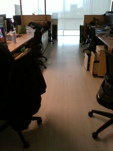
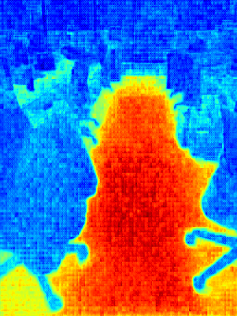
We run SAM-TP on an input image to predict traversable areas. The result is visualized as a color-coded heatmap, where:

🔴 Red regions are easier to navigate 🔵 Blue regions are harder to navigate

Input Image	Traversability Heatmap

If you use SAM-TP or the GeNIE system in your research, please cite our paper:

GeNIE: A Generalizable Navigation System for In-the-Wild Environments Jiaming Wang*, Diwen Liu*, Jizhuo Chen*, Jiaxuan Da, Nuowen Qian, Tram Minh Man, Harold Soh

@article{wang2024genie,
  title={GeNIE: A Generalizable Navigation System for In-the-Wild Environments},
  author={Wang, Jiaming and Liu, Diwen and Chen, Jizhuo and Da, Jiaxuan and Qian, Nuowen and Man, Tram Minh and Soh, Harold},
  journal={arXiv preprint arXiv:2506.17960},
  year={2024}
}